HOMEWORK 12 - SIMULATIONS
NOTE: Homework 12 is due after Thanksgiving break, on Wednesday Dec 2nd. Though this due
date is many days away, we highly, highly recommend that you get this assignment out of the
way sooner than later (which will then allow you to focus on your final project).
-- Christopher Parker
Simulations
As you well know by now, computers are GREAT at doing repetative tasks. In fact, they love it. So why not give your nice computer the thing it wants!? Until now, many of our repetative tasks have involved reading things from a file or performing simple calculations; in this homework assignment, you'll do something a little different. You're going to perform a simulation.
A lot of the time, a simulation depicts a complicated phenomenon that results from the interaction of numerous members in a system, all of which are behaving according to a simple set of rules. Computers are great for this type of work because it usually requires performing the same mathematical operation over and over again on the various members in the system. Moreover, since some simulations can take a long time to complete, a computer can perform a simulation for long periods of time and periodically output the 'current' state of the system (either visualizing it immediately on a screen or writing the necessary information to a file). A programmer (you!) can then watch the results of this simulation in action and, in turn, gain insight into why the original phenomenon occurs or how it can be used. Scientists and engineers perform simulations every day, so it is a very useful skill for you to learn how to do! The simulation that you will create for this homework is known as an N-Body simulation. These types of simulations depict the behavior of N (some number defined by the user) massive bodies in space. As you might expect, the only laws governing the behavior of these bodies in space is that of gravity and Newtonian mechanics (in 2-dimensions).
The final result of your homework will look similar to this:

Instructions
Download and extract this template. In the provided main.cpp file we have given you some default values to use (to be discussed below) as well as suggestions on where to place certain portions of your code. These constants are the default values we suggest you should use; you are welcome, however, to tailor them to your liking as you develop your code. This homework assignment consists of two parts: one that creates a body simulation identical to the one you visualized in Lab12A (in that the bodies do not interact with each other), and the second where the bodies are attracted to each other via gravity. For both of these parts you produce a simulation file that you can use your submission from Lab12A to visualize!
Part I: Implement a Body class
You will need to create a Body class which is capable of representing a massive body in space. We leave it to you to determine what properties and behaviors your Body class will need. We insist, however, that your properties are private (unless you can justify that a user needs direct access to a particular property); this means you will also need to create the mutator (setter) and accessor (getter) functions necessary to work with the properties. Two hints:
- Look at the equations below, which are necessary for this homework. You will likely need a property for each of the variables used in these equations (but not all).
- It would be a good idea to separate vector properties (such as position, velocity, and acceleration) into their X and Y components (for instance, X-Velocity and Y-Velocity).
Move() member function that will serve to update a body object's position in space according to that body's velocity. (FYI: Part I will not include acceleration, but Part II will.) This function should return a void and take at least one input argument, a change in time (Δt) in seconds, and possibly more depending on your needs. Updating the body object's position will be done using the kinematic equations with zero acceleration: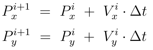
where:
- Pxi is the body's current X-position (m)
- Pyi is the body's current Y-position (m)
- Vxi is the body's current X-Velocity (m·s-1)
- Vyi is the body's current Y-Velocity (m·s-1)
- Pxi+1 is the body's new X-position (m)
- Pyi+1 is the body's new Y-position (m)
Move() function should also include a bouncing feature that checks the updated position of the body object to see if it has crossed one of the X or Y boundaries, e.g., your body object's X position must be between 0 and X Boundary. If your body object has moved outside the boundry, then you will need to flip the transgressive velocity (multiply by -1) so that the body returns to an acceptable position at the next time step of your simulation. For instance, suppose your X-boundary is 1000 and after updating a particular body's position the X-position is at 1002.35 with an X-velocity of 3.7. In order for the body to move back into acceptable space, its X-velocity must be multiplied by -1 (resulting in -3.7). This example illustrates how to implement the bouncing behavior needed in your simulation; we leave it to you to figure out the rest of the details.
Setup your simulation
Once you have your body class implemented, you need to do the following tasks before beginning your simulation:
- Ask the user how many bodies they would like to draw (lets call this number N)
- Construct N body objects (vector, maybe!?)
- Randomly initialize (within the suggested limits) the mass, positions, and velocities of each body
- body mass and X/Y positions must be greater than 0 and less than the respective maximums.
- body velocity should be within ±maximum velocity
- Ask the user how many time steps they would like to compute (e.g., 50000)
- Open an output file stream and write the two header lines into your file (see Lab12A for details on these header lines)
Perform your simulation
Once all of your bodies have been initialized and you know how many time steps your user would like to compute, you can begin your simulation. Create a loop that will iterate over each time step (called your simulation loop). Within that loop, do the following:
- Create another loop that calls the
Move()member function for each body - Check if the current iteration is a multiple of the provided constant
STEPS_PER_DRAW; if yes, write the current state of the system to your output file stream (discussed below)
Output File format
Your output file must follow the same format (our .bs format) that was used in Lab12A. As a reminder, it will look like the following, where your user chose to make 'N' bodies and run 'M * STEPS_PER_DRAW' time steps:
- Line 1: [N] [X Boundary] [Y Boundary]
- Line 2: [Body 1 size] [Body 2 size] [...] [Body N size]
- Line 3: [Body 1 X-Pos] [Body 1 Y-Pos] [Body 2 X-Pos] [Body 2 Y-Pos] [...] [Body N X-Pos] [Body N Y-Pos]
- Line 4: [Body 1 X-Pos] [Body 1 Y-Pos] [Body 2 X-Pos] [Body 2 Y-Pos] [...] [Body N X-Pos] [Body N Y-Pos]
- ...
- Line M: [Body 1 X-Pos] [Body 1 Y-Pos] [Body 2 X-Pos] [Body 2 Y-Pos] [...] [Body N X-Pos] [Body N Y-Pos]
Note: The second header line (i.e., the one that contains the size of each body) does not contain the mass of each body. Instead this line should contain the relative size of each body. That is, you should divide the mass of each individual body object by the maximum mass that is defined at the start of your program, resulting in values ranging from zero to one.
Part II
In the second part of this homework, you will update your Body class from the previous part to include gravitational interaction between the bodies. This is actually much easier than it sounds!
Update the Body Class
In order to accomplish this, you need to add a public CalculateAccelerationTo() member function that takes another Body object as an input. This function calculates the X/Y component accelerations of the callee's Body towards the input Body, add those components to the body's current X/Y acceleration, and returns a void. We provide a review of Newtonian Physics below, where we've provided the relevant equations; clearly you will have to convert these equations into C++. Also, be sure to implement the first bandaid fix that is discussed in the Computational Considerations section.
Secondly, you will need to update your Move() function such that the called body's X/Y positions are updated according to non-zero X/Y accelerations, followed by updating that body's X/Y velocities (in that order!). For this, you will update this function to use the kinematic equations with constant acceleration:
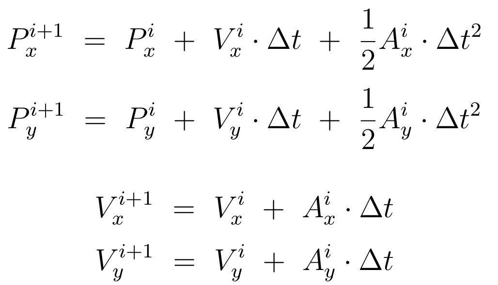
where (in addition to the variables mentioned previously):
- Axi is the summation of all X-Accelerations acting on the body for this time step
- Ayi is the summation of all Y-Accelerations acting on the body for this time step
- Vxi+1 is the body's new X-velocity
- Vyi+1 is the body's new Y-velocity
Move() function, which is discussed in the Computational Considerations section.
Updating the simulation loop
Within your simulation loop (before calling the Move() function for each body) you will need to calculate the total acceleration experienced by each body (which is a summation of all the individual accelerations toward the other bodies). This will require calling the CalculateAccelerationTo() function for each body using each of the other bodies as an input (hmmm ... I smell a nested for-loop). Hints: Do NOT calculate a body's acceleration towards itself and be sure to not include acceleration calculations from previous time steps. In total, you will need to call the CalculateAccelerationTo() function N*(N-1) times within each time step.
Simulation time!
Once all the above steps are done, then the position of your bodies will update as you would expect them to, and the state of your system will be written out to your output file in the same manner as before. You can then use the software you created in Lab12A to visualize your resulting simulation file. Nice!
As a final note, running your program for Part II will likely take a long time for a large number of bodies. This is expected since the way we are implementing this simulation is crude and very 'brute-force'. There are MANY things that could be done to improve the time this simulation takes to complete; alas, most of them are far outside the scope of this class. Nevertheless, if you can think of a clever way to improve the completion time of your simulation then don't hesitate to implement it! How many bodies can you draw!?
Newtonian Physics Review
For our N-Body simulation we will make use of Newton's Law of Universal Gravitation (why am I hungry for an apple all of a sudden?) which is summarized below:
Calculate total acceleration
Consider two bodies in space, labeled below as B1 and B2. In addition to the two bodies, the figure shows the total acceleration (in red) of B1 towards B2, the X/Y component accelerations of B1 (in green), and finally the X/Y component distances between the two objects (labeled dx and dy)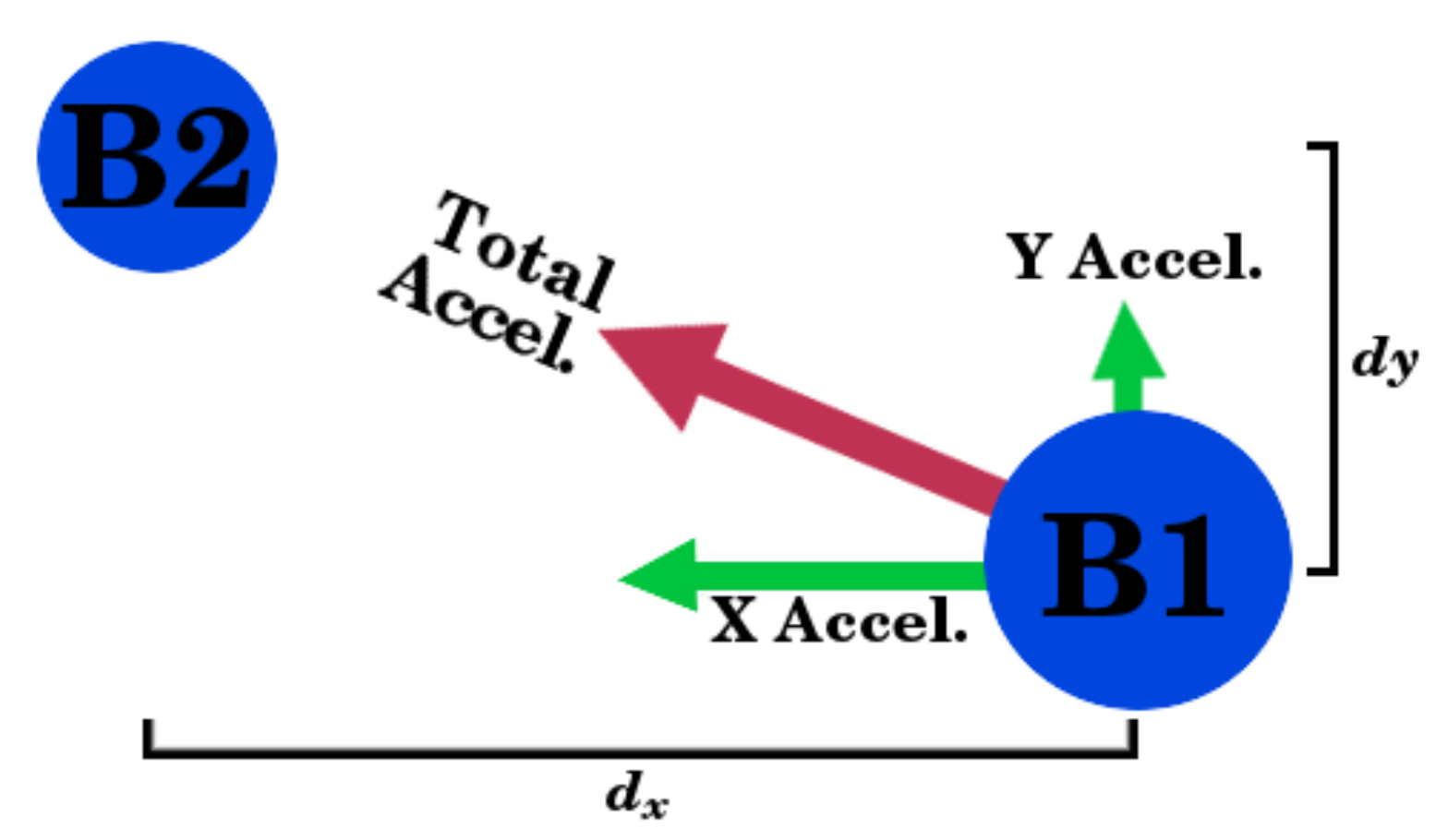
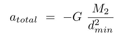
The total acceleration that the body B1 will experience in the direction of B2 can be calculated using:
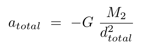
where:
- atotal is the magnitude of B1's acceleration towards B2 (m·s-2)
- G is the gravitational constant 6.67408×10⁻¹¹ m3·kg-1·s-2
- M2 is the mass of body B2 (kg)
- dtotal is the total distance between the two bodies (m)
Break the total acceleration into X/Y components
We will need to break up our total acceleration into X and Y component accelerations. This can be accomplished using: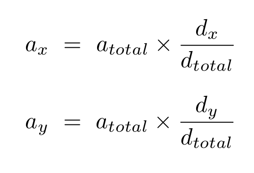
where:
- ax is the acceleration of B1 in the X-dimension
- ay is the acceleration of B1 in the Y-dimension
- dx is the difference of the bodies in the X-dimension
- dy is the difference of the bodies in the Y-dimension
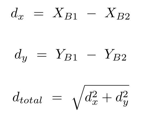
where:
- XB1 is the X-position of B1
- YB1 is the Y-position of B1
- XB2 is the X-position of B2
- YB2 is the Y-position of B2
Computational Considerations
Our computer will do a pretty good job of simulating our bodies in space, but it won't be perfect. The problem originates from instances where the instantaneous position and velocity are changing appreciably compared to the size of our time-step. There are many ways around this issue (the most effective being a "smart" time step); for our purposes, however, we will use two "bandaid fixes" (i.e., solutions that avoid an issue without actually fixing the underlying problem). These fixes only need to be applied to Part II of this assignment.
The first bandaid fix will impose a minimum calculable distance between our bodies. In the template you downloaded earlier we provide a suggested minimum distance (MIN_DISTANCE), which you are welcome to change to some other value if you want. When calculating the total distance between two bodies, if the resulting distance is larger than your minimum distance, then you should use the equation above for calculating total acceleration. However, if the resulting distance is found to be less than your minimum distance, then you should use the following equation for calculating total acceleration:
The second bandaid fix will impose a dampening effect onto our system. Whenever bodies bounce off the boundaries of the SFML window, you should reduce both component velocities by 75% (in addition to inverting the transgressive velocity).
Homework Grade and Submission
Your Homework 12 grade will be based on your solution to this assignment and your solution to Lab12A and Lab12B. In submitting your homework assignment (due Dec 2nd), follow these steps:
- create a directory called week12.
- within week12, create three subdirectories: Lab12A, Lab12B, and HW12.
- copy your main.cpp file from your Lab12A solution to your new week12/Lab12A directory.
- copy your main.cpp file from your Lab12B solution to your new week12/Lab12B directory.
- copy your main.cpp, your Body.cpp, and your your Body.h files from your HW12 solution to your new week12/HW12 directory.
- compress the week12 directory (see Step 3 here for details).
- submit the week12.zip file to Blackboard (see Steps 5-10 here for details).
- after you submit, download the file and double check it contains all that you think it contains!